When to use a vector database, when a SQL table, and when a graph, and what it costs to pick wrong

I asked my own system how many calls a week a voice agent I had built was handling. It came back with 600, and it had a source: a line in its own notes saying "600+ calls a week."

The tracker that number was summarising said about 1,850 a week, across 18 campaigns running at once. The note had been written once, early, and the real figure had tripled underneath it.

Nothing errored. No test went red. The search did exactly what it was built to do. It found the passage that best matched "how many calls a week," and that passage was a summary of a number rather than the number. A summary of a number is not the number, and there is nothing in a similarity score that can tell you which one you just got.

That is the failure this architecture exists to prevent. The fix was not a better search, and it was not a better model. It was noticing that the reader had changed.

For most of my career, data was modelled so that a person could read it. That is why tabular won. A human can scan a table, pivot it, put it on a dashboard, and apply the one reflex that matters here: hang on, is this figure still current? Star schemas, warehouses and BI tools were all built around human legibility.

The first consumer of the data I model now is an agent, and the human works through it. That changes the design question. It is no longer whether a person can navigate the store. It is what shape lets an agent retrieve the right slice cheaply, and not be confidently wrong when it cannot.

Why not just hand the model everything?

That is the honest baseline, and it deserves a straight answer rather than a hand-wave. If context were free and infinite, none of what follows would be worth building. You would pass all 1,100 documents to a frontier model with the question attached and take the answer.

It is not free, and that is the whole reason these architectures exist. Retrieval is a cost-minimisation exercise before it is anything else. Four of these files run 230 to 270 printed pages each; opening one to find a single figure costs roughly 180,000 tokens of reading. Eight typical lookups done that way come to 1,031,560 tokens. Answering the same eight from three narrow stores costs 16,290, and returns in about 17 milliseconds. That is 98% less, and it is paid per query, every query, forever.

Cost is the first reason and it is not the only one. Handing over everything would not have fixed the 600. Both numbers are in that archive: the stale summary and the tracker it summarised. A model given all of it sees both and has nothing to tell it which one is authoritative, because that fact is not in the text of either. More context does not adjudicate. It just moves the same ambiguity into a more expensive prompt.

So the goal is not the largest context you can afford. It is the smallest slice that is provably the right one, with each fact carrying where it came from.

Three things are being bought here, in that order of importance, and they are worth naming separately.

Fewer tokens. Tokens are the line item. A slice that is a hundredth the size costs a hundredth as much, on every single query, and that gap widens as the archive grows rather than closing.

Faster answers. A retrieval that returns in 17 milliseconds and hands over 16,000 tokens produces an answer in a fraction of the time a million-token prompt would, because the model has less to read before it can start.

Connections nobody thought to look for. This one is the graph's alone, it is not about cost, and it is the reason the third store exists at all. More on it below.

Against those two, each store does a specific job:

Store	What it removes	What it adds
Vector index	Reading whole documents. You scan the passages that match, not the file they sit in	Matching on meaning, so the right passage is found even when the question uses none of its words
Graph	A hand-written join for every hop, and having to think of the question first	Connections that surface on their own, including ones nobody would have known to ask for
SQL store	Nothing. It does exactly what it always did	Exact aggregation over rows, still the only correct way to produce a number

The last row is the one people skip past, and it is the most important. The tabular store is not the legacy layer being replaced by the two newer ones. Its job did not change at all. Counting is still counting, and a GROUP BY is still the right answer to "how many." What changed is that it stopped being the only store, because two of the three questions an agent asks were never countable in the first place.

The archive had three shapes, and one index over all of it was worse than three narrow ones

The material is about 1,100 documents: meeting notes, strategy decks, research logs, and several thousand spreadsheets. Four of the note files run 230 to 270 printed pages each. Before any of this existed, answering one factual question meant opening a whole document — roughly 180,000 tokens of reading to retrieve a single figure.

The obvious move is to chop everything into passages and embed the lot. That is the standard recipe, and on this archive it is wrong in a specific way.

Sort the same files by shape instead and three groups fall out.

Prose — anything written in sentences. Meeting notes, strategy documents, research write-ups. The useful question here is "what happened, and why," and the answer is a passage.

Grids — spreadsheets. The useful question is "how many," and the answer is a count over rows that no single passage contains.

Relationships — which investor backed which company, who worked where. The useful question needs more than one hop, and the answer is a path.

Each group goes to a different store. Prose to a local embedding index, grids to DuckDB, relationships to Kuzu. A fourth group — source code, media, financial and identity documents — goes nowhere at all.

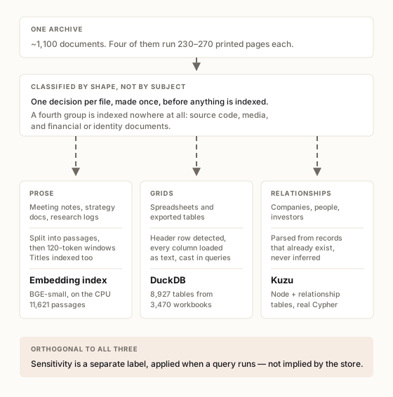
The current build is 11,621 passages and 54,459 smaller windows over the prose, plus 8,927 tables extracted from 3,470 workbooks. Eight typical lookups that would have cost 1,031,560 tokens of reading now cost 16,290, and come back in about 17 milliseconds. That is a 98% reduction, and almost none of it came from a cleverer model.

What a vector index is genuinely good at, measured against a baseline from the 1970s

A vector index converts each passage into a list of numbers — a point in space — so that passages about similar things land near each other. A question becomes a point too, and search is finding the nearest neighbours. The payoff is that it matches on meaning rather than words. Ask about a "migration" and it can find the passage that describes moving a reporting stack without ever using that word.

The honest question is whether that is worth the machinery. So I measured it against BM25, a keyword ranking function older than most of the people deploying vector databases. It needs no model, no GPU, and no index beyond a word-count table. On an archive full of proper nouns, BM25 is hard to beat.

Five methods over 38 hand-labelled questions:

Method	Correct answer ranked first	Found in top 10	Mean reciprocal rank
Plain word matching	49%	76%	0.585
BM25	51%	78%	0.615
Vector search	59%	81%	0.657
Small-to-big (default)	51%	84%	0.654
Vector + BM25 fused	57%	84%	0.656

Read that as a real, useful, unspectacular gain. Vector search puts the right answer first about eight percentage points more often than a decades-old keyword method. Worth having. Not the order-of-magnitude difference the category marketing implies.

Two findings mattered more than the choice of retriever.

Indexing each document's title alongside its passages moved keyword-search quality from 0.590 to 0.671 — on its own, nearly the entire gain the embedding model delivered, for no model and no cost. Several files state their whole subject in the filename and never repeat it in the body, so a passage indexed without its title was invisible to the obvious question. Fix what is inside the retrievable unit before shopping for a better retriever.

Match on small windows, return the big passage. A 500-token passage about process rules containing one clause with a metric in it gets that clause averaged into invisibility. So the index matches against roughly 120-token windows, where a single clause is a large share of the signal, and then hands back the parent passage so the reader still gets context. That is why the small-to-big row leads on top-10 recall despite a mediocre first-place score.

How to implement it. A 384-dimension sentence-transformer running on the CPU via ONNX, with no API call. An archive holding private material should not be shipped to a hosted embedding endpoint in a batch job. At this size the vectors are a 7.8 MB array file and search is one matrix multiplication, so a specialised vector database would add operating surface for no measurable speed gain. Two things are easy to get wrong. These models expect a specific instruction prefix on the query side and not the document side, and skipping it costs real accuracy. And vectors must be cached by a hash of the text, never by row position. A position-keyed cache silently pairs the wrong vector with the wrong passage. When passages were re-split mid-project and 267 were inserted, only 43% of the index still pointed at the text it was built for. It caught itself on a row-count check and fell back to keyword search loudly, which is the right behaviour — searching a misaligned index returns real, confidently scored, completely wrong passages.

A spreadsheet stops being a spreadsheet the moment you embed it

This is the counter-intuitive one, and it is where the 600-versus-1,850 error came from.

Chop a grid into paragraph-sized text and you destroy the rows and columns. What survives is a smear of numbers with their headers detached. "Which candidates reached the final round" is a GROUP BY, not a nearest-neighbour lookup. There is no passage anywhere that contains the answer, so the index does the only thing it can — it returns something that reads like the answer.

Worse, it degrades everything else in the index. Thousands of low-signal grid fragments sit in the same space competing with the prose that would have been useful. Embedding spreadsheets is the most common mistake in systems like this, and it damages both halves at once.

So grids go into DuckDB and are queried as tables. Three implementation choices carried their weight:

Load everything as text, and cast in the query. Real spreadsheets carry mixed types in one column — a date, a note, an empty string, an "N/A". Guessing a type per column either fails on load or silently discards data. Casting belongs in the query, where whoever wrote it can see the assumption.

Mirror the source of truth, never write back to it. The live tracker is owned by one small set of functions that snapshot before every save. The SQL store holds a read-only copy for querying. Two writers would break that contract.

Put restricted tables in a separate database file, not behind a flag. Some workbooks are hiring pipelines keyed to real people's names. They load, into a different file that has to be explicitly attached before any query can see it, and that attachment does not persist between sessions. A sensitivity column in the shared database would have been easier to build and would have put the burden on every query written afterwards. A convention is something you remember. A separate file is something you cannot forget.

A graph surfaces the connection nobody thought to ask for

Here is the question that justified the third store. Which company have I not approached yet that shares an investor with one where someone already replied?

That is a warm introduction instead of a cold approach, and it turns a long backlog into a short ranked list. It is also three joins deep. A table handles the first hop comfortably — list the investors in a given company. The second hop is where it turns awkward, and the second hop is the entire value.

A graph database stores entities as nodes and named, directed relationships as edges, both carrying their own properties. A company node holds a funding stage; the edge to its investor holds the round and the date. Traversal is following those edges: start somewhere you can name, walk a relationship type, arrive somewhere else, keep going. What comes back is a connected set of facts rather than a ranked list of passages.

Ask an embedding index that question and it does not fail loudly. It embeds the question, returns the passages that read most similarly, and none of them is the answer. Nothing errors, no score collapses, and nothing in the output indicates that the real answer needed specific edges walked instead. That is the characteristic failure of the whole category: the wrong store does not refuse, it improvises.

Cost and speed justify the first two stores. The graph earns its place on a different argument, and it is the one worth understanding, because it is the one people usually miss.

Work through a concrete case. I approach company A. Company A has an investor, call them X. X has also backed company B, which I had never heard of and would never have searched for. That link is not trivia. An investor backs along a thesis, so the fact that X funded both A and B says something real about B. It is the kind of company X believes in, which is very likely the kind of company I was already targeting when I picked A. Company B just became a lead, and a warm one, because someone now exists who knows both sides.

Every fact in that chain was already sitting in a tabular store. This is the part worth being precise about, because it is where the argument usually gets overstated: a relational database can absolutely answer this. Nothing is missing from the data. What is missing is the question.

To get company B out of a table, somebody first has to sit down, imagine that a shared investor might imply a shared thesis, and then write the self-join that walks from A to its investors to their other portfolio companies and back out. The insight has to exist in a human head before the query can be written. The database only confirms what somebody already suspected.

In a graph, nobody has to have the thought first. Company B falls out of an ordinary two-hop traversal from A, alongside every other company reachable the same way, because "follow this edge type, then follow it back" is simply how you move through the store rather than a clever thing you do to it. The structure does the imagining.

So the case for a graph is not cheaper queries. It is that a graph makes discovery the default. A table answers the question you thought to ask. A graph hands you connections you did not know were available, which is what you want in front of an agent that will not have a hunch on your behalf.

How to implement it. Kuzu, embedded — a directory on disk, no server, real Cypher. It requires a schema declared up front: node tables, relationship tables declared between specific pairs of node types, typed properties. That reads as friction while prototyping and turns out to be the most valuable property of the store.

Two rules, both learned the hard way:

Derive every edge from a record that already exists. Never infer one. A fabricated shared investor does not degrade an answer slightly — it manufactures a warm introduction that never existed and sends a real approach down it. This is a real divergence from how graph retrieval is usually built; the well-known approach has a model read the corpus and extract relationships. That is the right trade when relationships exist only in prose. It is the wrong one when a structured record exists and a wrong edge is expensive.

Refuse to create a node for a name you cannot match. Company names in written notes carry forms a tracking sheet does not. A parenthetical legal name, two names joined by a slash, a corporate suffix. Matching the literal string alone dropped eight companies' data silently, so lookup now tries a series of derived keys, most specific first. When a name still matches nothing, it is logged as unmatched and skipped. Inventing a company from a near-miss splits one company's edges across two nodes, and a traversal over a split node is confident and wrong.

The honest limit: this store is only as good as its coverage, and right now 14 of 113 companies have an investor recorded. A warm-introduction path needs a link on both ends, so the query mostly returns nothing. It says so, rather than returning a blank that reads like "there is nothing there." If you build this, add the field to your capture step on day one and report coverage as a number. A graph nobody fills in is an empty room with good architecture.

An instruction in a prompt is not a mechanism

All of the above is useless if the question reaches the wrong store, which brings us back to the 600.

The system's own written instructions already said numbers come from the spreadsheets. That is an instruction, and the search happily returned a paraphrase anyway, because an instruction sitting in a prompt does not constrain what a retriever does.

So a rule-based classifier now runs before anything is searched. A question asking for a quantity goes to SQL. A question asking for a reason goes to prose. A question naming two entities and asking what links them goes to the graph. A question needing a number and the story around it goes to two stores, and the results are labelled by origin.

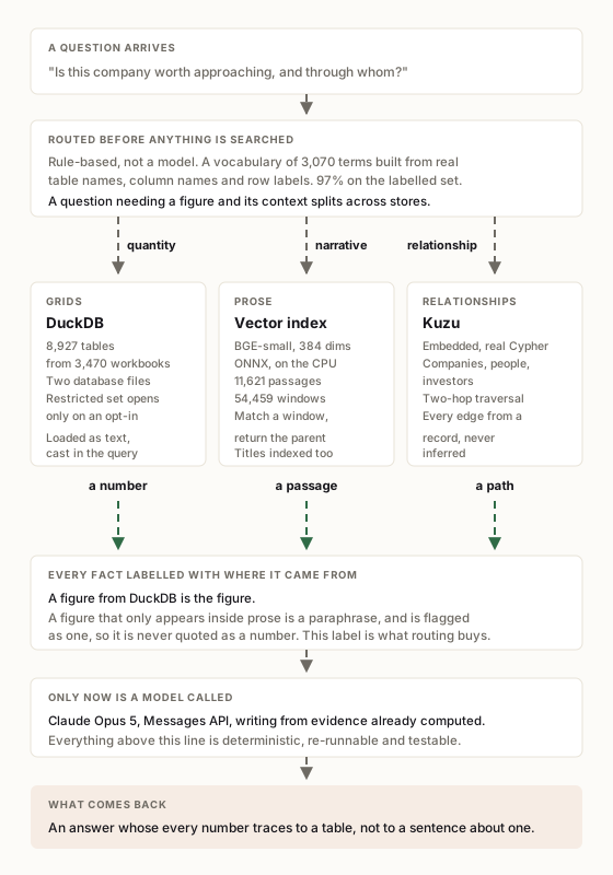
It is rule-based rather than model-based on purpose. Routing is a small, closed problem; a model classifier would be non-deterministic across runs and awkward to unit-test, and would make the retrieval layer depend on the thing it is supposed to be feeding. It scores 97% on the labelled question set and 12 of 14 on unseen phrasings, and both failures sent a question to SQL when prose was right — the harmless direction.

One implementation detail decides whether this works: the classifier is grounded in a 3,070-term vocabulary built at load time from actual table names, column names and row labels. Table names alone are far too weak. The table holding the call metrics contains neither "automation" nor "rate" in its name — those words are cell values. Build the vocabulary from the data, not from the schema.

When a question routes to SQL, the prose results still appear, under a warning that they are a paraphrase at best and must not be quoted as a figure. That warning is the difference between a draft citing your real results and a draft citing a stale note about them.

Three ingredients, one generation

Described one at a time, the three stores sound like alternatives you choose between. In a real request they are not alternatives. They run together, and each contributes something the other two cannot.

Take the outreach case end to end. The graph surfaces company B, which I did not know to ask about, through an investor it shares with a company already in play. The embedding index pulls the two or three paragraphs from my own archive that describe the work most relevant to what company B does, so the note cites something real rather than a generic claim. The tabular store supplies the exact figures that go in that note, drawn from the records that hold them rather than from a sentence about them.

Only then does a model get called, and what it receives is a small, labelled bundle: a connection worth acting on, the evidence that makes it credible, and numbers that are correct. It writes from that.

That combination is the actual argument for the architecture, and it moves four ways at once. The answer is more comprehensive, because it includes a lead no single store would have produced. It is more accurate, because every figure came from the store that holds figures. It is faster, because the model reads sixteen thousand tokens instead of a million. And it is cheaper, for the same reason.

Those four usually trade against each other. More comprehensive normally means more context, which means slower and more expensive. The reason they move together here is that the work of deciding what is relevant happened before the model was called, in three stores that are each cheap at their own job, rather than inside a single expensive prompt that was handed everything and asked to sort it out.

Where each store lets you stop a wrong answer

Choosing a store is usually framed as a performance question. In practice the more consequential difference is where each one lets you prevent a bad answer, because that determines who has to remember.

	Embedding index	SQL store	Graph
Question it makes cheap	Which passage explains this	How many rows match	What connects these two
Answer shape	A ranked list of passages	A number or a table	A path
Where prevention lives	A filter applied before ranking	A separate database file, attached on request	A relationship type that does not exist between those node types
Who has to remember	Every query path	Whoever writes the attach statement	Nobody
How it fails	A path forgets the filter, and the result looks normal	Someone attaches the restricted file and leaves it attached	The extraction writes an edge into the wrong table

Read the "who has to remember" row across. An embedding index can only filter, and every retrieval path has to carry that filter — a new path that forgets is a leak with no symptom. A SQL store can put restricted rows in a file that is not attached. A graph can go further: if two kinds of relationship are declared as separate relationship types, a query that names one cannot return the other, whether or not whoever wrote it thought about the distinction.

That mattered here for an ordinary reason. The archive mixes work contacts with personal ones, and a query looking for a former colleague must not return a personal contact. Rather than tag every person with a category and filter on it, the two kinds of connection are separate relationship types. The professional query names one of them, so the other is not reachable — not filtered out, unreachable.

The cost is that all the care moves to write time. A graph is defended once, by whoever decides which relationship type an edge belongs to, and everything downstream inherits that decision. Which is why the extraction rules that build it are deliberately strict, and why they are allowed to miss a real connection rather than guess at one.

One filter dimension applies to all three stores and is worth applying before the cutoff rather than after. Filter afterwards and an excluded row still consumes one of the five slots you asked for, so a query for five results quietly returns four.

Four employers wrote the same policy, and no retriever could tell them apart

One more finding, because it is the case where all three stores fail equally and the fix is in none of them.

The archive spans four employers, and each wrote an office policy, a leave policy and a contractor policy. The documents are near-identical in wording, because that is how such documents get written. Search matches on wording. Ask about one company's leave policy and that company's document ranked 16th under BM25 and 25th under vector search. The default returns five results. So the honest description is that it confidently handed back a different company's policy, with no indication anything was wrong.

Better search does not fix this, and it was worth measuring rather than assuming — the smarter method ranked the right answer worse than the crude one. The information needed to tell four near-identical documents apart was never in the text. It was in the file path: exported folders carry account names, and folder names carry company names.

So each document now carries an organisation label derived from where it sits rather than what it says, and a search can be scoped to one. Two properties of that label are worth copying. A document can carry several labels at once, because a contractor policy can sit in a second company's folder inside a third company's export and all three are true. And the label describes provenance, not subject matter — a note filed under one company that discusses another is labelled by where it lives. That is a real limit and the right trade, since labelling by content would match every document that so much as mentions a company, which is the problem being fixed.

One bug is worth recording, because it is the kind that hides. The machine's own user account is named after one of the companies. So the first version of the matcher matched every document in the archive, instead of the seventeen genuinely about that employer. There is now a test that fails if that ever stops being handled.

The pattern, without the job search

These architectures exist because tokens cost money and answers have to be fast. If context were free, one frontier model reading everything would win. It is not, so the job is to hand over the smallest slice that is provably right. A vector index means you stop reading whole documents. A graph means relationships become something you walk instead of reconstruct. A tabular store keeps doing what it always did, because counting never needed replacing. The engineering decision is not which database is best. It is which representation each question needs, and where that gets decided.

Domain	Goes to SQL	Goes to the vector index	Goes to the graph
Customer support	Tickets open past SLA this week	Find past tickets that read like this one	Why this account escalated three times running
Insurance claims	Average settlement by claim type	Find comparable prior claims	Trace this claim's reassignments and reopenings
Supply chain	Units short by SKU and region	Find comparable delayed shipments	Which upstream delay caused this stockout
Clinical operations	Readmissions within 30 days	Find similar case notes	Trace a patient's referral and readmission chain
Fraud investigation	Disputed volume by merchant	Find similarly worded disputes	Link two disputes by account, device and payment method
B2B sales	Pipeline by stage and owner	Find accounts with similar problems	Which prospect shares a board member with a closed customer

Three choices generalise past any of these.

Split the corpus by shape before you index anything. This is the decision that pays for itself, and it costs a day. Everything written in sentences goes one way, everything in rows and columns goes another, and everything that is neither goes nowhere. Teams reach for a better model when the actual problem is that a spreadsheet was chopped into paragraphs eight months ago and has been quietly poisoning retrieval ever since.

Put the routing decision in code, not in a prompt. "Numbers come from the database" is an instruction, and instructions do not constrain retrievers. A small rule-based classifier in front of the search decides before anything is retrieved, can be unit-tested, and gives the same answer twice. Score it on the same labelled question set as the retrieval itself, so a rule has to earn its place rather than just feel right.

Write the labelled question set before you build the retrieval layer. Thirty or forty real questions with known answers, written down. Without it, every choice above is unarguable in both directions: chunk size, whether to index titles, whether fusion helps, whether a graph is worth building. You will spend the budget on a bigger model instead of on the thing that was actually wrong.

A reference architecture, in build order

Start by classifying every source file by shape, with a sensitivity label decided separately and applied when a query runs rather than at ingest. Then the labelled question set, before any retrieval exists, because it is what makes every later choice arguable.

Then keyword search, as the baseline you have to beat. It costs an afternoon and on a corpus of proper nouns it is genuinely competitive. Index each document's title alongside its passages at this point — it is free and it closes most of the gap.

Then the embedding index, if the baseline is not enough. A small sentence- transformer on the CPU rather than a hosted endpoint, vectors cached by a hash of the text, matched against small windows and returning parent passages, in a plain array file until the corpus outgrows memory.

Then the SQL store for every grid, loaded as text and cast in the query, mirrored read-only from whatever owns the data, with restricted tables in a second database file that must be explicitly attached.

Then the graph, and only once a specific multi-hop question has a name. Model the edges that question actually walks rather than a speculative entity graph. Every edge derived from an existing record, never inferred. Distinctions that matter become separate relationship types rather than a property to filter on.

Finally the router in front of all three, rule-based, its vocabulary built from real table and column names, scored alongside retrieval.

Three things are cheap now and expensive later. Deciding which distinctions get their own relationship type before any edges exist, because splitting a merged one means re-typing every edge by hand. Keying the vector cache by content hash rather than row position from the first build, since the position-keyed version fails silently and plausibly. And capturing the fields a graph will need at the moment a record is created, because a graph with 12% coverage answers nothing no matter how well it is modelled.

References

Tooling

Kuzu — the embedded graph database used here. Its data model is "based on the property graph model, together with some structure (including node and relationship tables, and a pre-defined schema)", and that pre-declared schema is what turns a filtering convention into a structural guarantee.
DuckDB's ATTACH statement — how a restricted second database stays isolated. Attachment is explicit and not persisted between sessions: "when a new session is launched, you have to re-attach to all databases."
BAAI/bge-small-en-v1.5 — the 384-dimension, 33.4M-parameter embedding model behind the prose index, run locally on CPU, including the asymmetric query-side instruction prefix that is the easiest thing to get wrong when wiring one of these up.

Companion to Automating my job hunt outreach with an agent that finds, researches, and drafts, which covers the pipeline this memory layer sits under, and pgvector and Neo4j sitting on top of Postgres, which makes the same argument across three separate systems.